Notes on fastai Book Ch. 7
ai
fastai
notes
pytorch
Chapter 7 covers data normalization, progressive resizing, test-time augmentation, mixup, and label smoothing.
TipThis post is part of the following series:
- Training a State-of-the-Art Model
- Imagenette
- Normalization
- Progressive Resizing
- Test Time Augmentation
- Mixup
- Label Smoothing
- Papers and Math
- References
Training a State-of-the-Art Model
- the dataset you are given is not necessarily the dataset you want.
- aim to have an iteration speed of no more than a couple of minutes
- think about how you can cut down your dataset, or simplify your model to improve your experimentation speed
- the more experiments your can do the better
Imagenette
- https://docs.fast.ai/data.external.html
- A smaller version of the imagenet dataset
- Useful for quick experimentation and iteration
from fastai.vision.all import *path = untar_data(URLs.IMAGENETTE)
pathPath('/home/innom-dt/.fastai/data/imagenette2')parent_label
- https://docs.fast.ai/data.transforms.html#parent_label
- Label item with the parent folder name.
parent_label<function fastai.data.transforms.parent_label(o)>dblock = DataBlock(blocks=(
# TransformBlock for images
ImageBlock(),
# TransformBlock for single-label categorical target
CategoryBlock()),
# recursively load image files from path
get_items=get_image_files,
# label images using the parent folder name
get_y=parent_label,
# presize images to 460px
item_tfms=Resize(460),
# Batch resize to 224 and perform data augmentations
batch_tfms=aug_transforms(size=224, min_scale=0.75))
dls = dblock.dataloaders(path, bs=64, num_workers=8)xresnet50<function fastai.vision.models.xresnet.xresnet50(pretrained=False, **kwargs)>CrossEntropyLossFlat
- https://docs.fast.ai/losses.html#CrossEntropyLossFlat
- Same as
nn.CrossEntropyLoss, but flattens input and target.
CrossEntropyLossFlatfastai.losses.CrossEntropyLossFlat# Initialize the model without pretrained weights
model = xresnet50(n_out=dls.c)
learn = Learner(dls, model, loss_func=CrossEntropyLossFlat(), metrics=accuracy)
learn.fit_one_cycle(5, 3e-3)| epoch | train_loss | valid_loss | accuracy | time |
|---|---|---|---|---|
| 0 | 1.672769 | 3.459394 | 0.301718 | 00:59 |
| 1 | 1.224001 | 1.404229 | 0.552651 | 01:00 |
| 2 | 0.968035 | 0.996460 | 0.660941 | 01:00 |
| 3 | 0.699550 | 0.709341 | 0.771471 | 01:00 |
| 4 | 0.578120 | 0.571692 | 0.820388 | 01:00 |
# Initialize the model without pretrained weights
model = xresnet50(n_out=dls.c)
# Use mixed precision
learn = Learner(dls, model, loss_func=CrossEntropyLossFlat(), metrics=accuracy).to_fp16()
learn.fit_one_cycle(5, 3e-3)| epoch | train_loss | valid_loss | accuracy | time |
|---|---|---|---|---|
| 0 | 1.569645 | 3.962554 | 0.329724 | 00:33 |
| 1 | 1.239950 | 2.608771 | 0.355489 | 00:33 |
| 2 | 0.964794 | 0.982138 | 0.688200 | 00:34 |
| 3 | 0.721289 | 0.681677 | 0.791636 | 00:33 |
| 4 | 0.606473 | 0.581621 | 0.824122 | 00:33 |
Normalization
- normalized data: has a mean value of
0and a standard deviation of1 - it is easier to train models with normalized data
- normalization is especially important when using pretrained models
- make sure to use the same normalization stats the pretrained model was trained on
x,y = dls.one_batch()
x.mean(dim=[0,2,3]),x.std(dim=[0,2,3])
(TensorImage([0.4498, 0.4448, 0.4141], device='cuda:0'),
TensorImage([0.2893, 0.2792, 0.3022], device='cuda:0'))Normalize
- https://docs.fast.ai/data.transforms.html#Normalize
- Normalize/denormalize a bath of TensorImage
Normalizefastai.data.transforms.NormalizeNormalize.from_stats<bound method Normalize.from_stats of <class 'fastai.data.transforms.Normalize'>>def get_dls(bs, size):
dblock = DataBlock(blocks=(ImageBlock, CategoryBlock),
get_items=get_image_files,
get_y=parent_label,
item_tfms=Resize(460),
batch_tfms=[*aug_transforms(size=size, min_scale=0.75),
Normalize.from_stats(*imagenet_stats)])
return dblock.dataloaders(path, bs=bs)dls = get_dls(64, 224)x,y = dls.one_batch()
x.mean(dim=[0,2,3]),x.std(dim=[0,2,3])(TensorImage([-0.2055, -0.0843, 0.0192], device='cuda:0'),
TensorImage([1.1835, 1.1913, 1.2377], device='cuda:0'))model = xresnet50(n_out=dls.c)
learn = Learner(dls, model, loss_func=CrossEntropyLossFlat(), metrics=accuracy).to_fp16()
learn.fit_one_cycle(5, 3e-3)| epoch | train_loss | valid_loss | accuracy | time |
|---|---|---|---|---|
| 0 | 1.545518 | 3.255928 | 0.342046 | 00:35 |
| 1 | 1.234556 | 1.449043 | 0.560866 | 00:35 |
| 2 | 0.970857 | 1.310043 | 0.617252 | 00:35 |
| 3 | 0.736170 | 0.770678 | 0.758402 | 00:36 |
| 4 | 0.619965 | 0.575979 | 0.822629 | 00:36 |
Progressive Resizing
- start training with smaller images and end training with larger images
- gradually using larger and larger images as you train
- used by a team of fast.ai students to win the DAWNBench competition in 2018
- smaller images helps training complete much faster
- larger images helps makes accuracy much higher
- progressive resizing serves as another form of data augmentation
- should result in better generalization
- progressive resizing might hurt performance when using transfer learning
- most likely to happen if your pretrained model was very similar to your target task and the dataset it was trained on had similar-sized images
dls = get_dls(128, 128)
learn = Learner(dls, xresnet50(n_out=dls.c), loss_func=CrossEntropyLossFlat(),
                metrics=accuracy).to_fp16()
learn.fit_one_cycle(4, 3e-3)| epoch | train_loss | valid_loss | accuracy | time |
|---|---|---|---|---|
| 0 | 1.627504 | 2.495554 | 0.393951 | 00:21 |
| 1 | 1.264693 | 1.233987 | 0.613518 | 00:21 |
| 2 | 0.970736 | 0.958903 | 0.707618 | 00:21 |
| 3 | 0.740324 | 0.659166 | 0.794996 | 00:21 |
learn.dls = get_dls(64, 224)
learn.fine_tune(5, 1e-3)| epoch | train_loss | valid_loss | accuracy | time |
|---|---|---|---|---|
| 0 | 0.828744 | 1.024683 | 0.669529 | 00:36 |
| epoch | train_loss | valid_loss | accuracy | time |
|---|---|---|---|---|
| 0 | 0.670041 | 0.716627 | 0.776326 | 00:36 |
| 1 | 0.689798 | 0.706051 | 0.768857 | 00:36 |
| 2 | 0.589789 | 0.519608 | 0.831217 | 00:35 |
| 3 | 0.506784 | 0.436529 | 0.870426 | 00:36 |
| 4 | 0.453270 | 0.401451 | 0.877147 | 00:36 |
Test Time Augmentation
- during inference or validation, creating multiple versions of each image using augmentation, and then taking the average or maximum of the predictions for each augmented version of the image
- can result in dramatic improvements in accuracy, depending on the dataset
- does not change the time required to train
- will increase the amount of time required for validation or inference
Learner.tta
- https://docs.fast.ai/learner.html#Learner.tta
- returns predictions using Test Time Augmentation
learn.tta<bound method Learner.tta of <fastai.learner.Learner object at 0x7f75b4be5f40>>preds,targs = learn.tta()
accuracy(preds, targs).item()0.882001519203186Mixup
- a powerful data augmentation technique that can provide dramatically higher accuracy, especially when you don’t have much data and don’t have a pretrained model
- introduced in the 2017 paper mixup: Beyond Empirical Risk Minimization
- “While data augmentation consistently leads to improved generalization, the procedure is dataset-dependent, and thus requires the use of expert knowledge
- Mixup steps
- Select another image from your dataset at random
- Pick a weight at random
- Take a weighted average of the selected image with your image, to serve as your independent variable
- Take a weighted average of this image’s labels with your image’s labels, to server as your dependent variable
- target needs to be one-hot encoded
- \(\tilde{x} = \lambda x_{i} + (1 - \lambda) x_{j} \text{, where } x_{i} \text{ and } x_{j} \text{ are raw input vectors}\)
- \(\tilde{y} = \lambda y_{i} + (1 - \lambda) y_{j} \text{, where } y_{i} \text{ and } y_{j} \text{ are one-hot label encodings}\)
- more difficult to train
- less prone to overfitting
- requires far more epochs to to train to get better accuracy
- can be applied to types of data other than photos
- can even be used on activations inside of model
- resolves the issue where it is not typically possible to achieve a perfect loss score
- our labels are 1s and 0s, but the outputs of softmax and sigmoid can never equal 1 or 0
- with Mixup our labels will only be exactly 1 or 0 if two images from the same class are mixed
- Mixup is “accidentally” making the labels bigger than 0 or smaller than 1
- can be resolved with Label Smoothing
# Get two images from different classes
church = PILImage.create(get_image_files_sorted(path/'train'/'n03028079')[0])
gas = PILImage.create(get_image_files_sorted(path/'train'/'n03425413')[0])
# Resize images
church = church.resize((256,256))
gas = gas.resize((256,256))

# Scale pixel values to the range [0,1]
tchurch = tensor(church).float() / 255.
tgas = tensor(gas).float() / 255.

_,axs = plt.subplots(1, 3, figsize=(12,4))
# Show the first image
show_image(tchurch, ax=axs[0]);
# Show the second image
show_image(tgas, ax=axs[1]);
# Take the weighted average of the two images
show_image((0.3*tchurch + 0.7*tgas), ax=axs[2]);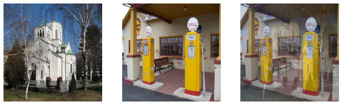
model = xresnet50()
learn = Learner(dls, model, loss_func=CrossEntropyLossFlat(), metrics=accuracy, cbs=MixUp).to_fp16()
learn.fit_one_cycle(15, 3e-3)| epoch | train_loss | valid_loss | accuracy | time |
|---|---|---|---|---|
| 0 | 2.332906 | 1.680691 | 0.431292 | 00:21 |
| 1 | 1.823880 | 1.699880 | 0.481329 | 00:21 |
| 2 | 1.660909 | 1.162998 | 0.650112 | 00:21 |
| 3 | 1.520751 | 1.302749 | 0.582524 | 00:21 |
| 4 | 1.391567 | 1.256566 | 0.595967 | 00:21 |
| 5 | 1.308175 | 1.193670 | 0.638163 | 00:21 |
| 6 | 1.224825 | 0.921357 | 0.706871 | 00:21 |
| 7 | 1.190292 | 0.846658 | 0.733383 | 00:21 |
| 8 | 1.124314 | 0.707856 | 0.780807 | 00:21 |
| 9 | 1.085013 | 0.701829 | 0.778193 | 00:21 |
| 10 | 1.028223 | 0.509176 | 0.851008 | 00:21 |
| 11 | 0.992827 | 0.518169 | 0.845780 | 00:21 |
| 12 | 0.945492 | 0.458248 | 0.864078 | 00:21 |
| 13 | 0.923450 | 0.418989 | 0.871546 | 00:21 |
| 14 | 0.904607 | 0.416422 | 0.876400 | 00:21 |
Label Smoothing
- Rethinking the Inception Architecture for Computer Vision
- in the theoretical expression of loss, in Classification problems, our targets are one-hot encoded
- the model is trained to return 0 for all categories but one, for which it is trained to return 1
- this encourages overfitting and gives your a model at inference time that is not going to give meaningful probabilities
- this can be harmful if your data is not perfectly labeled
- label smoothing: replace all our 1s with a number that is a bit less than 1, and our 0s with a number that is a bit more then 0
- encourages your model to be less confident
- makes your training more robust, even if there is mislabeled data
- results in a model that generalizes better at inference
- Steps
- start with one-hot encoded labels
- replace all 0s with \(\frac{\epsilon}{N}\) where \(N\) is the number of classes and \(\epsilon\) is a parameter (usually 0.1)
- replace all 1s with \(1 - \epsilon + \frac{\epsilon}{N}\) to make sure the labels add up to 1
model = xresnet50()
learn = Learner(dls, model, loss_func=LabelSmoothingCrossEntropy(), metrics=accuracy).to_fp16()
learn.fit_one_cycle(15, 3e-3)| epoch | train_loss | valid_loss | accuracy | time |
|---|---|---|---|---|
| 0 | 2.796061 | 2.399328 | 0.513443 | 00:21 |
| 1 | 2.335293 | 2.222970 | 0.584391 | 00:21 |
| 2 | 2.125152 | 2.478721 | 0.490291 | 00:21 |
| 3 | 1.967522 | 1.977260 | 0.690441 | 00:21 |
| 4 | 1.853788 | 1.861635 | 0.715459 | 00:21 |
| 5 | 1.747451 | 1.889759 | 0.699776 | 00:21 |
| 6 | 1.683000 | 1.710128 | 0.770351 | 00:21 |
| 7 | 1.610975 | 1.672254 | 0.780807 | 00:21 |
| 8 | 1.534964 | 1.691175 | 0.769231 | 00:21 |
| 9 | 1.480721 | 1.490685 | 0.842420 | 00:21 |
| 10 | 1.417200 | 1.463211 | 0.852502 | 00:21 |
| 11 | 1.360376 | 1.395671 | 0.867812 | 00:21 |
| 12 | 1.312882 | 1.360292 | 0.887603 | 00:21 |
| 13 | 1.283740 | 1.346170 | 0.890217 | 00:21 |
| 14 | 1.264030 | 1.339298 | 0.892830 | 00:21 |
Label Smoothing, Mixup and Progressive Resizing
dls = get_dls(128, 128)
model = xresnet50()
learn = Learner(dls, model, loss_func=LabelSmoothingCrossEntropy(), metrics=accuracy, cbs=MixUp).to_fp16()
learn.fit_one_cycle(15, 3e-3)| epoch | train_loss | valid_loss | accuracy | time |
|---|---|---|---|---|
| 0 | 3.045166 | 2.561215 | 0.449589 | 00:21 |
| 1 | 2.642317 | 2.906508 | 0.405900 | 00:21 |
| 2 | 2.473271 | 2.389416 | 0.516804 | 00:21 |
| 3 | 2.356234 | 2.263084 | 0.557506 | 00:21 |
| 4 | 2.268788 | 2.401770 | 0.544436 | 00:21 |
| 5 | 2.181318 | 2.040797 | 0.650485 | 00:21 |
| 6 | 2.122742 | 1.711615 | 0.761762 | 00:21 |
| 7 | 2.068317 | 1.961520 | 0.688200 | 00:21 |
| 8 | 2.022716 | 1.751058 | 0.743839 | 00:21 |
| 9 | 1.980203 | 1.635354 | 0.792009 | 00:21 |
| 10 | 1.943118 | 1.711313 | 0.758028 | 00:21 |
| 11 | 1.889408 | 1.454949 | 0.854742 | 00:21 |
| 12 | 1.853412 | 1.433971 | 0.862584 | 00:21 |
| 13 | 1.847395 | 1.412596 | 0.867438 | 00:22 |
| 14 | 1.817760 | 1.409608 | 0.875280 | 00:23 |
learn.dls = get_dls(64, 224)
learn.fine_tune(10, 1e-3)| epoch | train_loss | valid_loss | accuracy | time |
|---|---|---|---|---|
| 0 | 1.951753 | 1.672776 | 0.789395 | 00:36 |
| epoch | train_loss | valid_loss | accuracy | time |
|---|---|---|---|---|
| 0 | 1.872399 | 1.384301 | 0.892457 | 00:36 |
| 1 | 1.860005 | 1.441491 | 0.864078 | 00:36 |
| 2 | 1.876859 | 1.425859 | 0.867438 | 00:36 |
| 3 | 1.851872 | 1.460640 | 0.863331 | 00:36 |
| 4 | 1.840423 | 1.413441 | 0.880508 | 00:36 |
| 5 | 1.808990 | 1.444332 | 0.863704 | 00:36 |
| 6 | 1.777755 | 1.321098 | 0.910754 | 00:36 |
| 7 | 1.761589 | 1.312523 | 0.912621 | 00:36 |
| 8 | 1.756679 | 1.302988 | 0.919716 | 00:36 |
| 9 | 1.745481 | 1.304583 | 0.918969 | 00:36 |
Papers and Math
- Greek letters used in mathematics, science, and engineering
- Glossary of mathematical symbols
- Detexify
- draw a mathematical symbol and get the latex code
References
Previous: Notes on fastai Book Ch. 6
Next: Notes on fastai Book Ch. 8
TipAbout Me:
I’m Christian Mills, an Applied AI Consultant and Educator.
Whether I’m writing an in-depth tutorial or sharing detailed notes, my goal is the same: to bring clarity to complex topics and find practical, valuable insights.
If you need a strategic partner who brings this level of depth and systematic thinking to your AI project, I’m here to help. Let’s talk about de-risking your roadmap and building a real-world solution.
Start the conversation with my Quick AI Project Assessment or learn more about my approach.