Working with COCO Bounding Box Annotations in Torchvision
- Introduction
- Getting Started with the Code
- Setting Up Your Python Environment
- Importing the Required Dependencies
- Loading and Exploring the Dataset
- Preparing the Data
- Conclusion
Introduction
Welcome to this hands-on guide for working with COCO-formatted bounding box annotations in torchvision. Bounding box annotations specify rectangular frames around objects in images to identify and locate them for training object detection models.
The tutorial walks through setting up a Python environment, loading the raw annotations into a Pandas DataFrame, annotating and augmenting images using torchvision’s Transforms V2 API, and creating a custom Dataset class to feed samples to a model.
This guide is suitable for beginners and experienced practitioners, providing the code, explanations, and resources needed to understand and implement each step. By the end, you will have a solid foundation for working with COCO bounding box annotations in torchvision for object detection tasks.
Getting Started with the Code
The tutorial code is available as a Jupyter Notebook, which you can run locally or in a cloud-based environment like Google Colab. I have dedicated tutorials for those new to these platforms or who need guidance setting up:
| Jupyter Notebook: | GitHub Repository | Open In Colab |
|---|---|---|
Setting Up Your Python Environment
Before diving into the code, we’ll cover the steps to create a local Python environment and install the necessary dependencies.
Creating a Python Environment
First, we’ll create a Python environment using Conda/Mamba. Open a terminal with Conda/Mamba installed and run the following commands:
# Create a new Python 3.10 environment
conda create --name pytorch-env python=3.10 -y
# Activate the environment
conda activate pytorch-env
# Create a new Python 3.10 environment
mamba create --name pytorch-env python=3.10 -y
# Activate the environment
mamba activate pytorch-envInstalling PyTorch
Next, we’ll install PyTorch. Run the appropriate command for your hardware and operating system.
# Install PyTorch with CUDA
pip install torch torchvision torchaudio --index-url https://download.pytorch.org/whl/cu121
# MPS (Metal Performance Shaders) acceleration is available on MacOS 12.3+
pip install torch torchvision torchaudio# Install PyTorch for CPU only
pip install torch torchvision torchaudio --index-url https://download.pytorch.org/whl/cpu# Install PyTorch for CPU only
pip install torch torchvision torchaudioInstalling Additional Libraries
We also need to install some additional libraries for our project.
| Package | Description |
|---|---|
jupyter |
An open-source web application that allows you to create and share documents that contain live code, equations, visualizations, and narrative text. (link) |
matplotlib |
This package provides a comprehensive collection of visualization tools to create high-quality plots, charts, and graphs for data exploration and presentation. (link) |
pandas |
This package provides fast, powerful, and flexible data analysis and manipulation tools. (link) |
pillow |
The Python Imaging Library adds image processing capabilities. (link) |
tqdm |
A Python library that provides fast, extensible progress bars for loops and other iterable objects in Python. (link) |
distinctipy |
A lightweight python package providing functions to generate colours that are visually distinct from one another. (link) |
Run the following commands to install these additional libraries:
# Install additional dependencies
pip install distinctipy jupyter matplotlib pandas pillow tqdm
Installing Utility Packages
We will also install some utility packages I made, which provide shortcuts for routine tasks.
| Package | Description |
|---|---|
cjm_pil_utils |
Some PIL utility functions I frequently use. (link) |
cjm_psl_utils |
Some utility functions using the Python Standard Library. (link) |
cjm_pytorch_utils |
Some utility functions for working with PyTorch. (link) |
cjm_torchvision_tfms |
Some custom Torchvision tranforms. (link) |
Run the following commands to install the utility packages:
# Install additional utility packages
pip install cjm_pil_utils cjm_psl_utils cjm_pytorch_utils cjm_torchvision_tfms
With our environment set up, we can open our Jupyter Notebook and dive into the code.
Importing the Required Dependencies
First, we will import the necessary Python packages into our Jupyter Notebook.
# Import Python Standard Library dependencies
from functools import partial
from pathlib import Path

# Import utility functions
from cjm_pil_utils.core import get_img_files
from cjm_psl_utils.core import download_file, file_extract
from cjm_pytorch_utils.core import tensor_to_pil
from cjm_torchvision_tfms.core import ResizeMax, PadSquare, CustomRandomIoUCrop

# Import the distinctipy module
from distinctipy import distinctipy

# Import matplotlib for creating plots
import matplotlib.pyplot as plt

# Import numpy
import numpy as np

# Import the pandas package
import pandas as pd

# Do not truncate the contents of cells and display all rows and columns
pd.set_option('max_colwidth', None, 'display.max_rows', None, 'display.max_columns', None)

# Import PIL for image manipulation
from PIL import Image

# Import PyTorch dependencies
import torch
from torch.utils.data import Dataset, DataLoader

# Import torchvision dependencies
import torchvision
torchvision.disable_beta_transforms_warning()
from torchvision.tv_tensors import BoundingBoxes
from torchvision.utils import draw_bounding_boxes
import torchvision.transforms.v2  as transforms

# Import tqdm for progress bar
from tqdm.auto import tqdm
Torchvision provides dedicated torch.Tensor subclasses for different annotation types called TVTensors. Torchvision’s V2 transforms use these subclasses to update the annotations based on the applied image augmentations. The TVTensor class for bounding box annotations is called BoundingBoxes. Torchvision also includes a draw_bounding_boxes function to annotate images.
Loading and Exploring the Dataset
After importing the dependencies, we can start working with our data. I annotated a toy dataset with bounding boxes for this tutorial using images from the free stock photo site Pexels. The dataset is available on HuggingFace Hub at the link below:
- Dataset Repository: coco-bounding-box-toy-dataset
Setting the Directory Paths
We first need to specify a place to store our dataset and a location to download the zip file containing it. The following code creates the folders in the current directory (./). Update the path if that is not suitable for you.
# Define path to store datasets
dataset_dir = Path("./Datasets/")
# Create the dataset directory if it does not exist
dataset_dir.mkdir(parents=True, exist_ok=True)

# Define path to store archive files
archive_dir = dataset_dir/'../Archive'
# Create the archive directory if it does not exist
archive_dir.mkdir(parents=True, exist_ok=True)

# Creating a Series with the paths and converting it to a DataFrame for display
pd.Series({
    "Dataset Directory:": dataset_dir,
    "Archive Directory:": archive_dir
}).to_frame().style.hide(axis='columns')| Dataset Directory: | Datasets |
|---|---|
| Archive Directory: | Datasets/../Archive |
Setting the Dataset Path
Next, we construct the name for the Hugging Face Hub dataset and set where to download and extract the dataset.
# Set the name of the dataset
dataset_name = 'coco-bounding-box-toy-dataset'

# Construct the HuggingFace Hub dataset name by combining the username and dataset name
hf_dataset = f'cj-mills/{dataset_name}'

# Create the path to the zip file that contains the dataset
archive_path = Path(f'{archive_dir}/{dataset_name}.zip')

# Create the path to the directory where the dataset will be extracted
dataset_path = Path(f'{dataset_dir}/{dataset_name}')

# Creating a Series with the dataset name and paths and converting it to a DataFrame for display
pd.Series({
    "HuggingFace Dataset:": hf_dataset,
    "Archive Path:": archive_path,
    "Dataset Path:": dataset_path
}).to_frame().style.hide(axis='columns')| HuggingFace Dataset: | cj-mills/coco-bounding-box-toy-dataset |
|---|---|
| Archive Path: | Datasets/../Archive/coco-bounding-box-toy-dataset.zip |
| Dataset Path: | Datasets/coco-bounding-box-toy-dataset |
Downloading the Dataset
We can now download the archive file and extract the dataset using the download_file and file_extract functions from the cjm_psl_utils package. We can delete the archive afterward to save space.
# Construct the HuggingFace Hub dataset URL
dataset_url = f"https://huggingface.co/datasets/{hf_dataset}/resolve/main/{dataset_name}.zip"
print(f"HuggingFace Dataset URL: {dataset_url}")

# Set whether to delete the archive file after extracting the dataset
delete_archive = True

# Download the dataset if not present
if dataset_path.is_dir():
    print("Dataset folder already exists")
else:
    print("Downloading dataset...")
    download_file(dataset_url, archive_dir)

    print("Extracting dataset...")
    file_extract(fname=archive_path, dest=dataset_dir)

    # Delete the archive if specified
    if delete_archive: archive_path.unlink()
Getting the Image and Annotation Folders
The dataset has two folders containing the sample images and annotations. The image folder organizes all samples together. The annotations are in a single JSON file.
 # Assuming the images are stored in a subfolder named 'images'
img_dir = dataset_path/'images/'

# Assuming the annotation file is in JSON format and located in a subdirectory of the dataset
annotation_file_path = list(dataset_path.glob('*/*.json'))[0]

# Creating a Series with the paths and converting it to a DataFrame for display
pd.Series({
    "Image Folder": img_dir,
"Annotation File": annotation_file_path}).to_frame().style.hide(axis='columns')| Image Folder | Datasets/coco-bounding-box-toy-dataset/images |
|---|---|
| Annotation File | Datasets/coco-bounding-box-toy-dataset/annotations/instances_default.json |
Get Image File Paths
Each image file has a unique name that we can use to locate the corresponding annotation data. We can make a dictionary that maps image names to file paths. The dictionary will allow us to retrieve the file path for a given image more efficiently.
# Get all image files in the 'img_dir' directory
img_dict = {
    file.stem : file # Create a dictionary that maps file names to file paths
    for file in get_img_files(img_dir) # Get a list of image files in the image directory
}

# Print the number of image files
print(f"Number of Images: {len(img_dict)}")

# Display the first five entries from the dictionary using a Pandas DataFrame
pd.DataFrame.from_dict(img_dict, orient='index').head()
Number of Images: 28| 0 | |
|---|---|
| 258421 | Datasets/coco-bounding-box-toy-dataset/images/258421.jpg |
| 3075367 | Datasets/coco-bounding-box-toy-dataset/images/3075367.jpg |
| 3076319 | Datasets/coco-bounding-box-toy-dataset/images/3076319.jpg |
| 3145551 | Datasets/coco-bounding-box-toy-dataset/images/3145551.jpg |
| 3176048 | Datasets/coco-bounding-box-toy-dataset/images/3176048.jpg |
Get Image Annotations
Next, we read the content of the JSON annotation file into a Pandas DataFrame so we can easily query the annotations.
Load the annotation file into a DataFrame
We will transpose the DataFrame to store each section in the JSON file in a separate column.
# Read the JSON file into a DataFrame, assuming the JSON is oriented by index
annotation_file_df = pd.read_json(annotation_file_path, orient='index').transpose()
annotation_file_df.head()| licenses | info | categories | images | annotations | |
|---|---|---|---|---|---|
| 0 | {‘name’: ’‘, ’id’: 0, ‘url’: ’’} | contributor | {‘id’: 1, ‘name’: ‘person’, ‘supercategory’: ’’} | {‘id’: 1, ‘width’: 768, ‘height’: 1152, ‘file_name’: ‘258421.jpg’, ‘license’: 0, ‘flickr_url’: ’‘, ’coco_url’: ’‘, ’date_captured’: 0} | {‘id’: 1, ‘image_id’: 1, ‘category_id’: 1, ‘segmentation’: [], ‘area’: 24904.862800000003, ‘bbox’: [386.08, 443.94, 74.74, 333.22], ‘iscrowd’: 0, ‘attributes’: {‘occluded’: False, ‘rotation’: 0.0}} |
| 1 | None | date_created | None | {‘id’: 2, ‘width’: 1344, ‘height’: 768, ‘file_name’: ‘3075367.jpg’, ‘license’: 0, ‘flickr_url’: ’‘, ’coco_url’: ’‘, ’date_captured’: 0} | {‘id’: 2, ‘image_id’: 1, ‘category_id’: 1, ‘segmentation’: [], ‘area’: 24440.896000000004, ‘bbox’: [340.25, 466.94, 78.74, 310.4], ‘iscrowd’: 0, ‘attributes’: {‘occluded’: False, ‘rotation’: 0.0}} |
| 2 | None | description | None | {‘id’: 3, ‘width’: 768, ‘height’: 1120, ‘file_name’: ‘3076319.jpg’, ‘license’: 0, ‘flickr_url’: ’‘, ’coco_url’: ’‘, ’date_captured’: 0} | {‘id’: 3, ‘image_id’: 2, ‘category_id’: 1, ‘segmentation’: [], ‘area’: 365660.4554999999, ‘bbox’: [413.32, 41.22, 506.49, 721.95], ‘iscrowd’: 0, ‘attributes’: {‘occluded’: False, ‘rotation’: 0.0}} |
| 3 | None | url | None | {‘id’: 4, ‘width’: 1184, ‘height’: 768, ‘file_name’: ‘3145551.jpg’, ‘license’: 0, ‘flickr_url’: ’‘, ’coco_url’: ’‘, ’date_captured’: 0} | {‘id’: 4, ‘image_id’: 3, ‘category_id’: 1, ‘segmentation’: [], ‘area’: 363031.32340000005, ‘bbox’: [335.31, 151.75, 375.91, 965.74], ‘iscrowd’: 0, ‘attributes’: {‘occluded’: False, ‘rotation’: 0.0}} |
| 4 | None | version | None | {‘id’: 5, ‘width’: 1152, ‘height’: 768, ‘file_name’: ‘3176048.jpg’, ‘license’: 0, ‘flickr_url’: ’‘, ’coco_url’: ’‘, ’date_captured’: 0} | {‘id’: 5, ‘image_id’: 3, ‘category_id’: 1, ‘segmentation’: [], ‘area’: 390988.36079999997, ‘bbox’: [8.11, 131.88, 396.09, 987.12], ‘iscrowd’: 0, ‘attributes’: {‘occluded’: False, ‘rotation’: 0.0}} |
Let’s examine the source JSON content corresponding to the first row in the DataFrame.
{
    "licenses": [
        {
            "name": "",
            "id": 0,
            "url": ""
        }
    ],
    "info": {
        "contributor": "",
        "date_created": "",
        "description": "",
        "url": "",
        "version": "",
        "year": ""
    },
    "categories": [
        {
            "id": 1,
            "name": "person",
            "supercategory": ""
        }
    ],
    "images": [
        {
            "id": 1,
            "width": 768,
            "height": 1152,
            "file_name": "258421.jpg",
            "license": 0,
            "flickr_url": "",
            "coco_url": "",
            "date_captured": 0
        }
    ],
    "annotations": [
        {
            "id": 1,
            "image_id": 1,
            "category_id": 1,
            "segmentation": [],
            "area": 24904.862800000003,
            "bbox": [
                386.08,
                443.94,
                74.74,
                333.22
            ],
            "iscrowd": 0,
            "attributes": {
                "occluded": false,
                "rotation": 0.0
            }
        }
    ]
}
The most relevant information for our purposes is in the following sections:
categories: Stores the class names for the various object types in the dataset. Note that this toy dataset only has one object type.images: Stores the dimensions and file names for each image.annotations: Stores the image IDs, category IDs, and the bounding box annotations in[Top-Left X, Top-Left Y, Width, Height]format.
Extract the object classes
We first need to extract the class names from the categories column of the DataFrame.
# Extract and transform the 'categories' section of the data
# This DataFrame contains category details like category ID and name
categories_df = annotation_file_df['categories'].dropna().apply(pd.Series)
categories_df.set_index('id', inplace=True)
categories_df| name | supercategory | |
|---|---|---|
| id | ||
| 1 | person |
This toy dataset only contains a single object class, named person.
Extract the image information
Next, we will extract the file names, image dimensions, and Image IDs from the images column of the DataFrame.
# Extract and transform the 'images' section of the data
# This DataFrame contains image details like file name, height, width, and image ID
images_df = annotation_file_df['images'].to_frame()['images'].apply(pd.Series)[['file_name', 'height', 'width', 'id']]
images_df.head()| file_name | height | width | id | |
|---|---|---|---|---|
| 0 | 258421.jpg | 1152.0 | 768.0 | 1.0 |
| 1 | 3075367.jpg | 768.0 | 1344.0 | 2.0 |
| 2 | 3076319.jpg | 1120.0 | 768.0 | 3.0 |
| 3 | 3145551.jpg | 768.0 | 1184.0 | 4.0 |
| 4 | 3176048.jpg | 768.0 | 1152.0 | 5.0 |
Extract the annotation information
Last, we must extract the Image IDs, bounding box annotations, and Category IDs from the annotations column in the DataFrame.
# Extract and transform the 'annotations' section of the data
# This DataFrame contains annotation details like image ID, bounding box, and category ID
annotations_df = annotation_file_df['annotations'].to_frame()['annotations'].apply(pd.Series)[['image_id', 'bbox', 'category_id']]
annotations_df.head()| image_id | bbox | category_id | |
|---|---|---|---|
| 0 | 1 | [386.08, 443.94, 74.74, 333.22] | 1 |
| 1 | 1 | [340.25, 466.94, 78.74, 310.4] | 1 |
| 2 | 2 | [413.32, 41.22, 506.49, 721.95] | 1 |
| 3 | 3 | [335.31, 151.75, 375.91, 965.74] | 1 |
| 4 | 3 | [8.11, 131.88, 396.09, 987.12] | 1 |
Now that we have extracted the relevant information from the JSON file, we can recombine it into a single DataFrame for convenience.
Add the class names to the annotations
We will first add a new label column to the annotations_df DataFrame containing the corresponding class name from the categories_df DataFrame for each bounding box annotation.
# Map 'category_id' in annotations DataFrame to category name using categories DataFrame
annotations_df['label'] = annotations_df['category_id'].apply(lambda x: categories_df.loc[x]['name'])
annotations_df.head()| image_id | bbox | category_id | label | |
|---|---|---|---|---|
| 0 | 1 | [386.08, 443.94, 74.74, 333.22] | 1 | person |
| 1 | 1 | [340.25, 466.94, 78.74, 310.4] | 1 | person |
| 2 | 2 | [413.32, 41.22, 506.49, 721.95] | 1 | person |
| 3 | 3 | [335.31, 151.75, 375.91, 965.74] | 1 | person |
| 4 | 3 | [8.11, 131.88, 396.09, 987.12] | 1 | person |
Merge the image and annotation information
Next, we will add the data from the images_df DataFrame and match it to the bounding box annotations using the Image IDs.
# Merge annotations DataFrame with images DataFrame on their image ID
annotation_df = pd.merge(annotations_df, images_df, left_on='image_id', right_on='id')
annotation_df.head()| image_id | bbox | category_id | label | file_name | height | width | id | |
|---|---|---|---|---|---|---|---|---|
| 0 | 1 | [386.08, 443.94, 74.74, 333.22] | 1 | person | 258421.jpg | 1152.0 | 768.0 | 1.0 |
| 1 | 1 | [340.25, 466.94, 78.74, 310.4] | 1 | person | 258421.jpg | 1152.0 | 768.0 | 1.0 |
| 2 | 2 | [413.32, 41.22, 506.49, 721.95] | 1 | person | 3075367.jpg | 768.0 | 1344.0 | 2.0 |
| 3 | 3 | [335.31, 151.75, 375.91, 965.74] | 1 | person | 3076319.jpg | 1120.0 | 768.0 | 3.0 |
| 4 | 3 | [8.11, 131.88, 396.09, 987.12] | 1 | person | 3076319.jpg | 1120.0 | 768.0 | 3.0 |
Use the image name as the index
Then, we will change the index for the annotations_df DataFrame to match the keys in the img_dict dictionary, allowing us to retrieve both the image paths and annotation data using the same index key.
# Remove old 'id' column post-merge
annotation_df.drop('id', axis=1, inplace=True)

# Extract the image_id from the file_name (assuming file_name contains the image_id)
annotation_df['image_id'] = annotation_df['file_name'].apply(lambda x: x.split('.')[0])

# Set 'image_id' as the index for the DataFrame
annotation_df.set_index('image_id', inplace=True)
annotation_df.head()| bbox | category_id | label | file_name | height | width | |
|---|---|---|---|---|---|---|
| image_id | ||||||
| 258421 | [386.08, 443.94, 74.74, 333.22] | 1 | person | 258421.jpg | 1152.0 | 768.0 |
| 258421 | [340.25, 466.94, 78.74, 310.4] | 1 | person | 258421.jpg | 1152.0 | 768.0 |
| 3075367 | [413.32, 41.22, 506.49, 721.95] | 1 | person | 3075367.jpg | 768.0 | 1344.0 |
| 3076319 | [335.31, 151.75, 375.91, 965.74] | 1 | person | 3076319.jpg | 1120.0 | 768.0 |
| 3076319 | [8.11, 131.88, 396.09, 987.12] | 1 | person | 3076319.jpg | 1120.0 | 768.0 |
Group annotations by image
Each bounding box annotation is currently in a separate row in the DataFrame. We will want to group the annotations for each image into a single row for use with PyTorch and torchvision.
# Group the data by 'image_id' and aggregate information
# This results in each image ID having a list of bounding boxes, category IDs, labels, and the respective file name, height, and width
annotation_df = annotation_df.groupby('image_id').agg({'bbox': list,
                                           'category_id': list,
                                           'label' :list,
                                           'file_name': 'first',
                                           'height': 'first',
                                           'width': 'first'
                                                      })

# Rename columns for clarity
# 'bbox' is renamed to 'bboxes' and 'label' to 'labels'
annotation_df.rename(columns={'bbox': 'bboxes', 'label': 'labels'}, inplace=True)
annotation_df.head()| bboxes | category_id | labels | file_name | height | width | |
|---|---|---|---|---|---|---|
| image_id | ||||||
| 258421 | [[386.08, 443.94, 74.74, 333.22], [340.25, 466.94, 78.74, 310.4]] | [1, 1] | [person, person] | 258421.jpg | 1152.0 | 768.0 |
| 3075367 | [[413.32, 41.22, 506.49, 721.95]] | [1] | [person] | 3075367.jpg | 768.0 | 1344.0 |
| 3076319 | [[335.31, 151.75, 375.91, 965.74], [8.11, 131.88, 396.09, 987.12]] | [1, 1] | [person, person] | 3076319.jpg | 1120.0 | 768.0 |
| 3145551 | [[642.0, 289.85, 27.66, 109.04], [658.63, 281.25, 28.46, 117.36]] | [1, 1] | [person, person] | 3145551.jpg | 768.0 | 1184.0 |
| 3176048 | [[518.23, 338.97, 76.4, 127.11], [683.42, 356.48, -44.56, 81.34]] | [1, 1] | [person, person] | 3176048.jpg | 768.0 | 1152.0 |
With the annotations loaded, we can start inspecting our dataset.
Inspecting the Class Distribution
First, we get the names of all the classes in our dataset and inspect the distribution of samples among these classes. This step won’t yield any insights for the toy dataset but is worth doing for real-world projects. A balanced dataset (where each class has approximately the same number of instances) is ideal for training a machine-learning model.
Get image classes
# Get a list of unique labels in the 'annotation_df' DataFrame
class_names = annotation_df['labels'].explode().unique().tolist()

# Display labels using a Pandas DataFrame
pd.DataFrame(class_names)| 0 | |
|---|---|
| 0 | person |
Visualize the class distribution
# Get the number of samples for each object class
class_counts = pd.DataFrame(annotation_df['labels'].explode().tolist()).value_counts()

plot_labels = [index[0] for index in class_counts.index]

# Plot the distribution
class_counts.plot(kind='bar', figsize=(12, 5))
plt.title('Class distribution')
plt.ylabel('Count')
plt.xlabel('Classes')
plt.xticks(range(len(class_counts.index)), plot_labels, rotation=75)  # Set the x-axis tick labels
plt.show()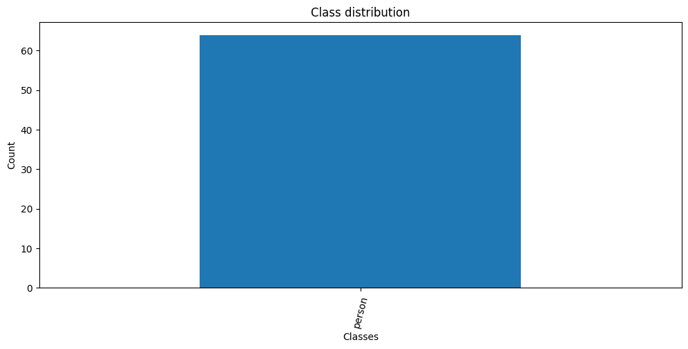
Visualizing Image Annotations
In this section, we will annotate a single image with its bounding boxes using torchvision’s BoundingBoxes class and draw_bounding_boxes function.
Generate a color map
While not required, assigning a unique color to bounding boxes for each object class enhances visual distinction, allowing for easier identification of different objects in the scene. We can use the distinctipy package to generate a visually distinct colormap.
# Generate a list of colors with a length equal to the number of labels
colors = distinctipy.get_colors(len(class_names))

# Make a copy of the color map in integer format
int_colors = [tuple(int(c*255) for c in color) for color in colors]

# Generate a color swatch to visualize the color map
distinctipy.color_swatch(colors)
Download a font file
The draw_bounding_boxes function included with torchvision uses a pretty small font size. We can increase the font size if we use a custom font. Font files are available on sites like Google Fonts, or we can use one included with the operating system.
# Set the name of the font file
font_file = 'KFOlCnqEu92Fr1MmEU9vAw.ttf'

# Download the font file
download_file(f"https://fonts.gstatic.com/s/roboto/v30/{font_file}", "./")
Define the bounding box annotation function
We can make a partial function using draw_bounding_boxes since we’ll use the same box thickness and font each time we visualize bounding boxes.
draw_bboxes = partial(draw_bounding_boxes, fill=False, width=2, font=font_file, font_size=25)Selecting a Sample Image
We can use the unique ID for an image in the image dictionary to get the image file path and the associated annotations from the annotation DataFrame.
Load the sample image
# Get the file ID of the first image file
file_id = list(img_dict.keys())[0]

# Open the associated image file as a RGB image
sample_img = Image.open(img_dict[file_id]).convert('RGB')

# Print the dimensions of the image
print(f"Image Dims: {sample_img.size}")

# Show the image
sample_img
Image Dims: (768, 1152)
Inspect the corresponding annotation data
# Get the row from the 'annotation_df' DataFrame corresponding to the 'file_id'
annotation_df.loc[file_id].to_frame()| 258421 | |
|---|---|
| bboxes | [[386.08, 443.94, 74.74, 333.22], [340.25, 466.94, 78.74, 310.4]] |
| category_id | [1, 1] |
| labels | [person, person] |
| file_name | 258421.jpg |
| height | 1152.0 |
| width | 768.0 |
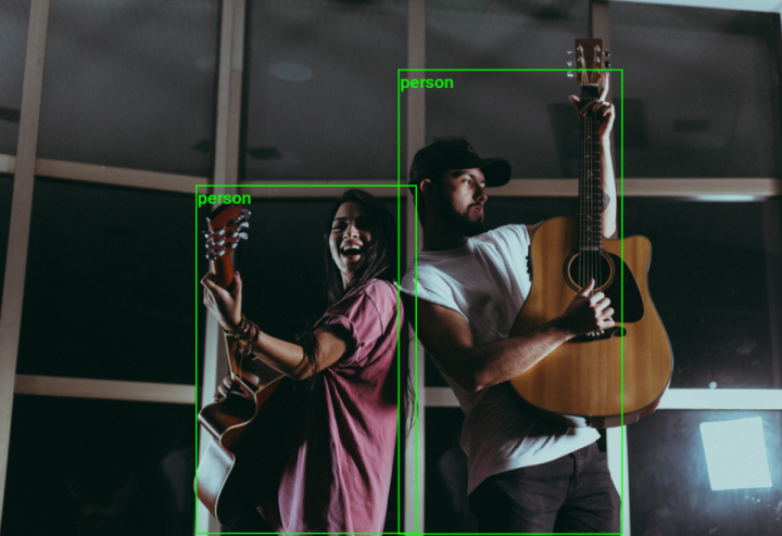
Annotate sample image
The draw_bounding_boxes function expects bounding box annotations in [top-left X, top-left Y, bottom-right X, bottom-right Y] format, so we’ll use the box_convert function included with torchvision to convert the bounding box annotations from [x,y,w,h] to [x,y,x,y] format.
# Extract the labels and bounding box annotations for the sample image
labels = annotation_df.loc[file_id]['labels']
bboxes = annotation_df.loc[file_id]['bboxes']

# Annotate the sample image with labels and bounding boxes
annotated_tensor = draw_bboxes(
    image=transforms.PILToTensor()(sample_img),
    boxes=torchvision.ops.box_convert(torch.Tensor(bboxes), 'xywh', 'xyxy'),
    labels=labels,
    colors=[int_colors[i] for i in [class_names.index(label) for label in labels]]
)

tensor_to_pil(annotated_tensor)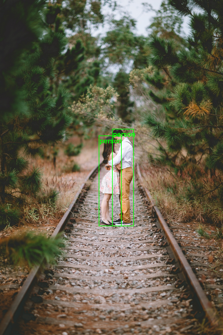
We have loaded the dataset, inspected its class distribution, and visualized the annotations for a sample image. In the final section, we will cover how to augment images using torchvision’s Transforms V2 API and create a custom Dataset class for training.
Preparing the Data
In this section, we will first walk through a single example of how to apply augmentations to a single annotated image using torchvision’s Transforms V2 API before putting everything together in a custom Dataset class.
Data Augmentation
Here, we will define some data augmentations to apply to images during training. I created a few custom image transforms to help streamline the code.
The first extends the RandomIoUCrop transform included with torchvision to give the user more control over how much it crops into bounding box areas. The second resizes images based on their largest dimension rather than their smallest. The third applies square padding and allows the padding to be applied equally on both sides or randomly split between the two sides.
All three are available through the cjm-torchvision-tfms package.
Set training image size
Next, we will specify the image size to use during training.
# Set training image size
train_sz = 384
Initialize custom transforms
Now, we can initialize the transform objects.
# Create a RandomIoUCrop object
iou_crop = CustomRandomIoUCrop(min_scale=0.3,
                               max_scale=1.0,
                               min_aspect_ratio=0.5,
                               max_aspect_ratio=2.0,
                               sampler_options=[0.0, 0.1, 0.3, 0.5, 0.7, 0.9, 1.0],
                               trials=400,
                               jitter_factor=0.25)

# Create a `ResizeMax` object
resize_max = ResizeMax(max_sz=train_sz)

# Create a `PadSquare` object
pad_square = PadSquare(shift=True)
Test the transforms
Torchvision’s V2 image transforms take an image and a targets dictionary. The targets dictionary contains the annotations and labels for the image.
We will pass input through the CustomRandomIoUCrop transform first and then through ResizeMax and PadSquare. We can pass the result through a final resize operation to ensure both sides match the train_sz value.
# Prepare bounding box targets
targets = {
    'boxes': BoundingBoxes(torchvision.ops.box_convert(torch.Tensor(bboxes), 'xywh', 'xyxy'),
                           format='xyxy',
                           canvas_size=sample_img.size[::-1]),
    'labels': torch.Tensor([class_names.index(label) for label in labels])
}

# Crop the image
cropped_img, targets = iou_crop(sample_img, targets)

# Resize the image
resized_img, targets = resize_max(cropped_img, targets)

# Pad the image
padded_img, targets = pad_square(resized_img, targets)

# Ensure the padded image is the target size
resize = transforms.Resize([train_sz] * 2, antialias=True)
resized_padded_img, targets = resize(padded_img, targets)
sanitized_img, targets = transforms.SanitizeBoundingBoxes()(resized_padded_img, targets)

# Annotate the augmented image with updated labels and bounding boxes
annotated_tensor = draw_bboxes(
    image=transforms.PILToTensor()(sanitized_img),
    boxes=targets['boxes'],
    labels=[class_names[int(label.item())] for label in targets['labels']],
    colors=[int_colors[i] for i in [class_names.index(label) for label in labels]]
)

# Display the annotated image
display(tensor_to_pil(annotated_tensor))

pd.Series({
    "Source Image:": sample_img.size,
    "Cropped Image:": cropped_img.size,
    "Resized Image:": resized_img.size,
    "Padded Image:": padded_img.size,
    "Resized Padded Image:": resized_padded_img.size,
}).to_frame().style.hide(axis='columns')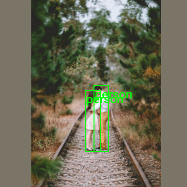
| Source Image: | (768, 1152) |
|---|---|
| Cropped Image: | (653, 941) |
| Resized Image: | (266, 383) |
| Padded Image: | (383, 383) |
| Resized Padded Image: | (384, 384) |
Now that we know how to apply data augmentations, we can put all the steps we’ve covered into a custom Dataset class.
Training Dataset Class
The following custom Dataset class is responsible for loading a single image, preparing the associated annotations, applying any image transforms, and returning the final image tensor and its target dictionary during training.
class COCOBBoxDataset(Dataset):
    """
    A dataset class for COCO-style datasets with bounding box annotations.

    This class is designed to handle datasets where images are annotated with bounding boxes,
    such as object detection tasks. It supports loading images, applying transformations,
    and retrieving the associated bounding box annotations.

    Attributes:
        _img_keys (list): A list of keys (identifiers) for each image in the dataset.
        _annotation_df (DataFrame): A DataFrame containing annotations for the images.
                                    Each row corresponds to an image, indexed by its key.
        _img_dict (dict): A dictionary mapping image keys to their file paths.
        _class_to_idx (dict): A dictionary mapping class names to their corresponding indices.
        _transforms (callable, optional): Optional transform to be applied on a sample.

    Methods:
        __len__: Returns the number of images in the dataset.
        __getitem__: Retrieves an image and its corresponding target (bounding boxes and labels)
                     by index.
        _load_image_and_target: Helper function to load an image and its corresponding target.
    """

    def __init__(self, img_keys, annotation_df, img_dict, class_to_idx, transforms=None):
        """
        Initializes the COCOBBoxDataset instance.

        Parameters:
            img_keys (list): List of image keys.
            annotation_df (DataFrame): DataFrame containing image annotations.
            img_dict (dict): Dictionary mapping image keys to file paths.
            class_to_idx (dict): Dictionary mapping class names to indices.
            transforms (callable, optional): Optional transform to be applied on a sample.
        """
        super(Dataset, self).__init__()

        self._img_keys = img_keys  # List of image keys
        self._annotation_df = annotation_df  # DataFrame containing annotations
        self._img_dict = img_dict  # Dictionary mapping image keys to image paths
        self._class_to_idx = class_to_idx  # Dictionary mapping class names to class indices
        self._transforms = transforms  # Image transforms to be applied

    def __len__(self):
        """
        Returns the total number of images in the dataset.

        Returns:
            int: The number of images in the dataset.
        """
        return len(self._img_keys)

    def __getitem__(self, index):
        """
        Retrieves an image and its corresponding target (bounding boxes and labels) by index.

        Parameters:
            index (int): The index of the image in the dataset.

        Returns:
            tuple: A tuple containing the image and its target. The target is a dictionary with
                   keys 'boxes' and 'labels'.
        """
        img_key = self._img_keys[index]
        annotation = self._annotation_df.loc[img_key]
        image, target = self._load_image_and_target(annotation)

        if self._transforms:
            # Apply the specified transformations to the image and target
            image, target = self._transforms(image, target)

        return image, target

    def _load_image_and_target(self, annotation):
        """
        Helper function to load an image and its corresponding target.

        The target includes bounding boxes and labels for the image.

        Parameters:
            annotation (pandas.Series): The annotation data for the image, typically a row from the DataFrame.

        Returns:
            tuple: A tuple containing the image and its target, where the target is a dictionary
                   with keys 'boxes' and 'labels'.
        """
        # Load the image file using the path from the image dictionary
        filepath = self._img_dict[annotation.name]
        image = Image.open(filepath).convert('RGB')

        # Extract bounding box data from the annotations and convert to the desired format
        bbox_list = annotation['bboxes']
        bbox_tensor = torchvision.ops.box_convert(torch.Tensor(bbox_list), 'xywh', 'xyxy')
        boxes = BoundingBoxes(bbox_tensor, format='xyxy', canvas_size=image.size[::-1])

        # Convert class labels in the annotation to their corresponding indices
        annotation_labels = annotation['labels']
        labels = torch.Tensor([self._class_to_idx[label] for label in annotation_labels])

        return image, {'boxes': boxes, 'labels': labels}
Image Transforms
Here, we will specify and organize all the image transforms to apply during training.
# Compose transforms for data augmentation
data_aug_tfms = transforms.Compose(
    transforms=[
        iou_crop,
        transforms.ColorJitter(
                brightness = (0.875, 1.125),
                contrast = (0.5, 1.5),
                saturation = (0.5, 1.5),
                hue = (-0.05, 0.05),
        ),
        transforms.RandomGrayscale(),
        transforms.RandomEqualize(),
        transforms.RandomPosterize(bits=3, p=0.5),
        transforms.RandomHorizontalFlip(p=0.5),
    ],
)

# Compose transforms to resize and pad input images
resize_pad_tfm = transforms.Compose([
    resize_max,
    pad_square,
    transforms.Resize([train_sz] * 2, antialias=True)
])

# Compose transforms to sanitize bounding boxes and normalize input data
final_tfms = transforms.Compose([
    transforms.ToImage(),
    transforms.ToDtype(torch.float32, scale=True),
    transforms.SanitizeBoundingBoxes(),
])

# Define the transformations for training and validation datasets
train_tfms = transforms.Compose([
    data_aug_tfms,
    resize_pad_tfm,
    final_tfms
])Always use the SanitizeBoundingBoxes transform to clean up annotations after using data augmentations that alter bounding boxes (e.g., cropping, warping, etc.).
Initialize Dataset
Now, we can create the dataset object using the image dictionary, the annotation DataFrame, and the image transforms.
# Create a mapping from class names to class indices
class_to_idx = {c: i for i, c in enumerate(class_names)}

# Instantiate the dataset using the defined transformations
train_dataset = COCOBBoxDataset(list(img_dict.keys()), annotation_df, img_dict, class_to_idx, train_tfms)

# Print the number of samples in the training dataset
pd.Series({
    'Training dataset size:': len(train_dataset),
}).to_frame().style.hide(axis='columns')| Training dataset size: | 28 |
|---|
Inspect Samples
To close out, we should verify the dataset object works as intended by inspecting the first sample.
Inspect training set sample
dataset_sample = train_dataset[0]

annotated_tensor = draw_bboxes(
    image=(dataset_sample[0]*255).to(dtype=torch.uint8),
    boxes=dataset_sample[1]['boxes'],
    labels=[class_names[int(i.item())] for i in dataset_sample[1]['labels']],
    colors=[int_colors[int(i.item())] for i in dataset_sample[1]['labels']]
)

tensor_to_pil(annotated_tensor)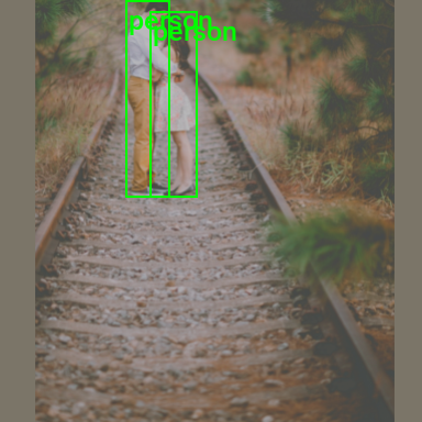
Conclusion
In this tutorial, we covered how to load custom COCO bounding box annotations and work with them using torchvision’s Transforms V2 API. The skills and knowledge you acquired here provide a solid foundation for future object detection projects.
As a next step, perhaps try annotating a custom COCO object detection dataset with a tool like CVAT and loading it with this tutorial’s code. Once you’re comfortable with that, try adapting the code in the following tutorial to train an object detection model on your custom dataset.
Recommended Tutorials
- Working with COCO Segmentation Annotations in Torchvision: Learn how to work with COCO segmentation annotations in torchvision for instance segmentation tasks.
- Training YOLOX Models for Real-Time Object Detection in PyTorch: Learn how to train YOLOX models for real-time object detection in PyTorch by creating a hand gesture detection model.
- Feel free to post questions or problems related to this tutorial in the comments below. I try to make time to address them on Thursdays and Fridays.
I’m Christian Mills, an Applied AI Consultant and Educator.
Whether I’m writing an in-depth tutorial or sharing detailed notes, my goal is the same: to bring clarity to complex topics and find practical, valuable insights.
If you need a strategic partner who brings this level of depth and systematic thinking to your AI project, I’m here to help. Let’s talk about de-risking your roadmap and building a real-world solution.
Start the conversation with my Quick AI Project Assessment or learn more about my approach.