GPU MODE Lecture 12: Flash Attention

Lecture #12 provides an introduction to Flash Attention, a highly optimized CUDA kernel for accelerating attention computations in transformer models, including a conceptual overview, tiling strategy, softmax stabilization, and limitations.

This post is part of the following series:

• GPU MODE Lecture Notes: My notes from the GPU MODE reading group lectures run by Andreas Kopf and Mark Saroufim.

• Introduction
• Background: The Need for Optimization
• Memory Hierarchy and Performance
• Attention Mechanisms: A Brief Overview
• Flash Attention: Tiling Strategy
• The Softmax Challenge
• Flash Attention 2: Advanced Techniques
• Implementation Attempts and Challenges
• CUDA C++ Implementation
• Performance Evaluation and Future Directions
• Conclusion
• Q&A Session

Resource Links:

• YouTube Recording: Lecture 12: Flash Attention

Introduction

• Presenter: Thomas Viehmann
• Topic: Flash Attention, a highly optimized CUDA kernel for attention mechanisms in AI models, specifically transformers.
• Focus: This lecture provides an introductory overview of Flash Attention, its underlying principles, and implementation challenges. It does not delve into live coding of the fastest kernels due to time constraints.

Background: The Need for Optimization

• Attention Mechanisms: Attention mechanisms are computationally intensive and memory-demanding operations in transformer models.
• Optimizing for Performance: Flash Attention aims to optimize attention calculations by:
  • Minimizing data transfers between DRAM (main memory) and SRAM (on-chip memory).
  • Leveraging the speed advantages of SRAM over DRAM (typically an order of magnitude faster).
  • Reducing memory allocation and holding times, addressing GPU memory limitations.

Memory Hierarchy and Performance

• DRAM vs. SRAM:
  • DRAM: Larger capacity but slower access times.
  • SRAM (Shared Memory): Smaller capacity but significantly faster access times.
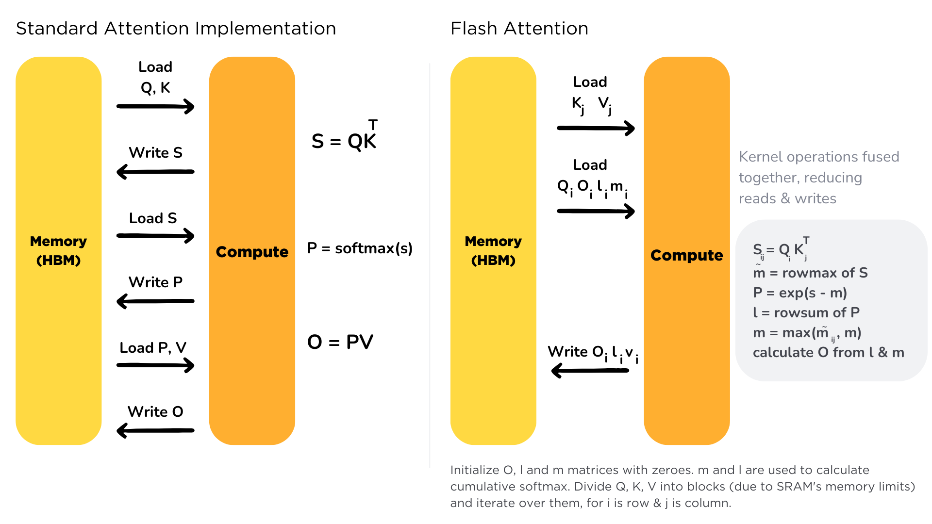
• Minimizing DRAM Access: Flash Attention focuses on reducing the need to write intermediate results to DRAM and then reload them, aiming to keep computations within SRAM as much as possible.
• Changes in GPU Computing: GPU architectures and software have evolved, requiring more sophisticated optimization techniques compared to earlier approaches where simple kernel sequencing could saturate GPU utilization.

Attention Mechanisms: A Brief Overview

• Attention as Classification: Attention can be viewed as a classification process within a neural network.

  • Analogy to Classification Heads: Similar to a classification head in a network, attention involves:
    • Input activations (d-dimensional): \(q\)
    • A final layer (\(K\)) producing logits: \(l = q K^T\)
    • Softmax function to generate probabilities: \(p_i = \frac{\exp(l_i)}{\sum_j \exp(l_j)}\)

• Class Embeddings Perspective: The final linear layer (K) can be interpreted as class embeddings. Each row of the matrix represents an embedding of a target class.

  • Input activations (d-dimensional): \(q\)
  • Class embeddings (d-dimensional): \(K = (k_i)\)
  • Logits: \(l_i = q \cdot k_i\)
  • Class Probabilities: \(p_i = \frac{\exp(d^{-1/2} l_i)}{\sum_j \exp(d^{-1/2} l_j)}\)

• Attention Weights: Attention weights are derived from scalar products of these embeddings, followed by a softmax operation to produce probabilities. \[ q_t = Qx_t, w_s = Kx_s \]

• Multi-Head Attention:

  • Multiple Classifications: Multi-head attention performs multiple independent classifications simultaneously, each with a smaller dimension (d).
  • Benefits:
    • Representational Power: Allows the model to attend to information from different representation subspaces and positions (as stated in the “Attention is All You Need” paper).
    • Computational Simplification: Heads are independent, enabling easy parallelization across the batch dimension and multiple streaming multiprocessors (SMs).

• Mapping to GPU Hardware:

  • One Head per Block: Flash Attention typically maps the computation of one attention head to a single block of threads on the GPU.
  • Blocks and SMs: A block of threads is processed by one SM. The goal is to have enough blocks to utilize all available SMs on the GPU.
  • Shared Memory: Threads within a block can share memory, making it efficient to store and access data needed for the attention head’s computation.

• Head Dimension Constraint: The size of the head dimension (d) is a limiting factor as it affects the amount of shared memory and registers required per block. Flash Attention implementations often use small, fixed head dimensions (e.g., 128 or 256) to ensure computations fit within the resources of a single SM.

Flash Attention: Tiling Strategy

• Computing One Output Element: The core idea is to analyze the computation required for a single element of the output matrix. \[ O[t, d] \]

• Output Element Dependencies:

  • Requires values (V) for all sequence elements (s) and the hidden dimension (d). \[ V[s, d] \text{ for all } s \]

  • Requires softmax probabilities (P) for the specific output sequence element (t) and all sequence elements (s). \[ \text{softmax}(I[t, s], \text{dim}=-1) \text{ for } t \rightarrow \text{need } I[t, s] = \sum_d Q[t, d] \text{ } K[s, d] \]

• Softmax and Contraction Dimension Alignment: Crucially, the dimension over which the softmax is computed (s) is the same as the contraction dimension between the softmax output and the value matrix (V). This enables efficient tiling.

• Tiling Scheme:

  for t_tile:
      load(Q[t_tile]) to shared, init O[t, d] = 0
      for s_tile:
          load(K[s_tile], V[s_tile]) to shared;
          compute I[t, s] = Q[t_tile] @ K^T[s_tile]  (compute p[t, s])
          O[t, d] += p[t_tile, s_tile] @ V[s_tile]
      write O[t, d]

  • Tiling in Output Dimension (t): The output dimension is tiled into blocks.
  • Loading Query Tile: A corresponding query tile (Q) is loaded into shared memory, covering the entire hidden dimension (d).
  • Iterating over Sequence Tiles (s): An inner loop iterates over tiles in the sequence dimension (s).
  • Loading Key and Value Tiles: For each s-tile, the corresponding key (K) and value (V) tiles are loaded into shared memory.
  • Computing Logits and Probabilities: The logits (L) and probabilities (P) are computed for the Q-tile and K-tile using matrix multiplication.
  • Updating Output: The output tile is updated by multiplying the computed probability matrix with the V-tile.
  • Writing Output Tile: Once the inner loop is complete, the output tile is written back to memory.

• HuggingFace text-generation-inference Docs: Flash Attention

  

  Standard Attention vs Flash Attention v1

The Softmax Challenge

• Softmax Formula:
  • \(p_i = exp(l_i) / \sum_j(exp(l_j))\)
  • \(p\): probabilities, \(l\): logits
• Numerical Stability: The exponential function can lead to very large or small values, causing numerical instability in the softmax calculation.
  • PyTorch Dev Discussions: FMAs (and softmax (and floating point)) considered harmful
• Stabilized Softmax:
  • Stabilization Technique: The softmax is stabilized by subtracting the maximum logit (m) from all logits before exponentiation.
  • \(p_i = exp(l_i - m) / \sum_j(exp(l_j - m))\)
  • Benefits: Ensures that the numerator values are between 0 and 1, improving numerical stability.
• Online Softmax:
  • Incremental Update: The stabilized softmax can be computed incrementally by adjusting the sum when the maximum logit (m) changes.
  • Implementation: Flash Attention often implements this online softmax block-by-block.

Flash Attention 2: Advanced Techniques

• Flash Attention 1 vs. 2: Flash Attention 2 significantly improves performance over Flash Attention 1 by avoiding writing intermediate results (O, L, M) to DRAM.
• Key Features:
  • Masking Support: Handles non-rectangular block layouts for masked attention.
  • Optimized Tile Ordering: Rearranges tile processing order to minimize DRAM writes.
  • CUTLASS Integration: Leverages the NVIDIA CUTLASS library for efficient tensor core utilization in matrix multiplications.
• Compilation Challenges: The integration of CUTLASS makes Flash Attention 2 a complex C++ codebase, leading to significant compilation time and memory requirements.

Implementation Attempts and Challenges

• Triton Tutorial: Fused Attention

• Manual PyTorch Implementation:

  import torch, math
  
  # within one block.
  N_inp = 64
  N_out = 64
  d = 128
  
  Q = torch.randn(N_out, d)
  K = torch.randn(N_inp, d)
  V = torch.randn(N_inp, d)
  O = torch.zeros(N_out, d)
  L = torch.zeros(N_out, 1)
  
  B_c = 16
  B_r = 16
  T_c = (N_inp + B_c - 1) // B_c
  T_r = (N_out + B_r - 1) // B_r
  
  scale_factor = 1 / math.sqrt(Q.size(-1))
  
  # Q and O split into T_r; K, V in T_c blocks
  for i in range(T_r):
      Q_i = Q[i * B_r: (i + 1) * B_r]
      O_i = torch.zeros(B_r, d)
      L_i = torch.zeros(B_r, 1)
      m_i = torch.full((B_r, 1), -math.inf)
      last_m_i = m_i
  
      for j in range(T_c):
          K_j = K[j * B_c: (j + 1) * B_c]
          V_j = V[j * B_c: (j + 1) * B_c]
          S_ij = scale_factor * (Q_i @ K_j.T)
          m_i = torch.maximum(m_i, S_ij.max(dim=-1, keepdim=True).values)
          P_ij = torch.exp(S_ij - m_i)
          P_ij = torch.exp(last_m_i - m_i) * L_i + P_ij.sum(dim=-1, keepdim=True)
          O_i = torch.exp(last_m_i - m_i) * O_i + P_ij @ V_j
          L_i = P_ij
  
      last_m_i = m_i
      O[i * B_r: (i + 1) * B_r] = O_i
      L[i * B_r: (i + 1) * B_r] = L_i

• Numba Implementation: Initial attempts to implement Flash Attention in Numba (a Python-based CUDA kernel compiler) encountered limitations with shared memory capacity, especially for larger tile sizes.

  pip install numba

  import numba.cuda
  
  @numba.cuda.jit
  def attention(K, Q, V, scaling: numba.float32, L, O):
      inp_dtype = K.dtype
      tid_x = numba.cuda.threadIdx.x
      tid_y = numba.cuda.threadIdx.y
  
      # Shared memory arrays
      Q_i = numba.cuda.shared.array((B_r, d), inp_dtype)
      K_j = numba.cuda.shared.array((B_c, d), inp_dtype)
      V_j = numba.cuda.shared.array((B_c, d), inp_dtype)
      O_i = numba.cuda.shared.array((B_r, d), inp_dtype)
      L_i = numba.cuda.shared.array((B_r, 1), inp_dtype)
      m_i = numba.cuda.shared.array((B_r, 1), inp_dtype)
      S_ij = numba.cuda.shared.array((B_c,), inp_dtype)
  
      for i in range(T_r):
          for ii in range(tid_y, B_r, numba.cuda.blockDim.y):
              for dd in range(tid_x, d, numba.cuda.blockDim.x):
                  Q_i[ii, dd] = Q[ii + i * B_r, dd]
                  O_i[ii, dd] = 0
              L_i[ii] = 0
              m_i[ii] = -math.inf
          numba.cuda.syncthreads()
  
          for j in range(T_c):
              for jj in range(tid_y, B_c, numba.cuda.blockDim.y):
                  for dd in range(tid_x, d, numba.cuda.blockDim.x):
                      K_j[jj, dd] = K[jj + j * B_c, dd]
                      V_j[jj, dd] = V[jj + j * B_c, dd]
              numba.cuda.syncthreads()
  
              # S_ij = scale_factor * (Q_i @ K_j.T)
              for ii in range(tid_x, B_r, numba.cuda.blockDim.x):
                  numba.cuda.syncthreads()
  
                  for jj in range(tid_y, B_c, numba.cuda.blockDim.y):
                      S_ij = 0
                      for dd in range(d):
                          S_ij += Q_i[ii, dd] * K_j[jj, dd]
                      S_ij = scale_factor * S_ij
                      S_ij_store[jj] = S_ij
  
                  # m_i = torch.maximum(m_i, S_ij.max(dim=-1, keepdim=True).values)
                  # This needs to use the parallel reduction pattern
                  numba.cuda.syncthreads()
  
                  m = m_i[ii]
                  last_m = m
  
                  for jj in range(B_c):
                      m = max(m, S_ij_store[jj])
                  m_i[ii] = m
                  L_i[ii] = math.exp(last_m - m) * L_i[ii]
  
                  numba.cuda.syncthreads()
  
                  for dd in range(d):
                      O_i[ii, dd] *= math.exp(last_m - m)
  
                  for jj in range(B_c):
                      S_ij_store[jj] = math.exp(S_ij_store[jj] - m)  # Cache the value
                      for dd in range(d):
                          O_i[ii, dd] += S_ij_store[jj] * V_j[jj, dd]
  
                  L_i[ii] = L_i[ii]
  
          for ii in range(tid_y, B_r, numba.cuda.blockDim.y):
              for dd in range(tid_x, d, numba.cuda.blockDim.x):
                  O[ii + i * B_r, dd] = O_i[ii, dd] / L_i[ii]
              L[ii + i * B_r] = L_i[ii]

  # Initialization code
  O2 = torch.zeros(N_out, d, device="cuda")
  L2 = torch.zeros(N_out, device="cuda")
  Kc = K.to("cuda")
  Qc = Q.to("cuda")
  Vc = V.to("cuda")
  
  # Call to the attention kernel
  attention((32, 4), (1,))(Kc, Qc, Vc, scale_factor, L2, O2)

• Shared Memory vs. Registers:

  • Shared Memory: Typically used for Q, K, and V matrices.
  • Registers: Ideally used for intermediate results like logits (L), probabilities (P), and outputs (O) to maximize speed.

• Register Allocation in CUDA: CUDA can automatically allocate variables to registers if they are:

  • Declared as local arrays with constant size.
  • Accessed using simple loop indices (not dynamic indices).

CUDA C++ Implementation

pip install cuda-python

from cuda import cuda, nvrtc

cuda_src = r"""\

constexpr int B_r = 16;
constexpr int B_c = 16;
constexpr int d = 128;
constexpr int o_per_thread_x = 1;
constexpr int o_per_thread_y = 128 / 32;

#define NEG_INFINITY __int_as_float(0xff800000)

extern "C" __global__
void silly_attn(float *out, float *out_l, float *K, float *Q, float *V, float scaling, int n, int T_r, int T_c) 
{
    int tid_x = threadIdx.x;
    int tid_y = threadIdx.y;
    __shared__ float Q_i[B_r][d];
    __shared__ float K_j[B_c][d];
    __shared__ float V_j[B_c][d];

    __shared__ float S_i[B_r][B_c];

    float l_i[o_per_thread_x];
    float m_i[o_per_thread_x];
    float O_i[o_per_thread_x][o_per_thread_y];

    for (int i = 0; i < T_r; i++) {
        for (int ii = 0; ii < o_per_thread_x; ii++) {
            for (int dd = 0; dd < o_per_thread_y; dd++) {
                O_i[ii][dd] = 0;
            }
            l_i[ii] = 0.f;
            m_i[ii] = NEG_INFINITY;
        }
        
        for (int ii = tid_y; ii < B_r; ii += blockDim.y) {
            for (int dd = tid_x; dd < d; dd += blockDim.x) {
                Q_i[ii][dd] = Q[(ii + i * B_r) * d + dd];
            }
        }
        
        for (int j = 0; j < T_c; j++) {
            __syncthreads();
            for (int jj = tid_y; jj < B_c; jj += blockDim.y) {
                for (int dd = tid_x; dd < d; dd += blockDim.x) {
                    K_j[jj][dd] = K[(jj + j * B_c) * d + dd];
                    V_j[jj][dd] = V[(jj + j * B_c) * d + dd];
                }
            }
            __syncthreads();
            // S_i = scale_factor * (Q_i @ K_j.T);
            for (int ii = tid_x; ii < B_r; ii += blockDim.x) {
                for (int jj = tid_y; jj < B_c; jj += blockDim.y) {
                    float S_ij = 0.f;
                    for (int dd = 0; dd < d; dd++) {
                        S_ij += Q_i[ii][dd] * K_j[jj][dd];
                    }
                    S_ij = scaling * S_ij;
                    S_i[ii][jj] = S_ij;
                }
            }
            __syncthreads();
            for (int ii = 0; ii < o_per_thread_x; ii++) {
                float m = m_i[ii];
                float last_m = m;
                for (int jj = 0; jj < B_c; jj+=1) {
                    if (m < S_i[ii] * blockDim.x + tid_x[jj]) {
                        m = S_i[ii] * blockDim.x + tid_x[jj];
                    }
                }
                m_i[ii] = m;
                float l = exp(last_m - m) * l_i[ii];
                for (int dd = 0; dd < o_per_thread_y; dd++) {
                    O_i[ii][dd] *= exp(last_m - m);
                }
            
                for (int jj = 0; jj < B_c; jj++) {
                    float S_ij = exp(S_i[ii] * blockDim.x + tid_x[jj] - m);
                    l += S_ij;
                    for (int dd = 0; dd < o_per_thread_y; dd++) {
                        O_i[ii][dd] += S_ij * V_j[jj][dd + blockDim.y + tid_y];
                    }
                }
                l_i[ii] = l;
                
            }
        }
        for (int ii = 0; ii < o_per_thread_x; ii++) {
            for (int dd = 0; dd < o_per_thread_y; dd++) {
                out[(ii * blockDim.x + tid_x + i * B_r) * d + dd * blockDim.y + tid_y] = O_i[ii][dd] / l_i[ii];
                out_l[ii * blockDim.x + tid_x + i * B_r] = l_i[ii];
            }
        }
    }
}
"""

# Create program
err, prog = nvrtc.nvrtcCreateProgram(str.encode(cuda_src), b"silly_attn.cu", 0, [], [])

# Compile program
min, maj = torch.cuda.get_device_capability()
opts = [f"--gpu-architecture=compute_{min}{maj}".encode()]
err, = nvrtc.nvrtcCompileProgram(prog, len(opts), opts)

print(err)

# Get PTX from compilation
err, ptxSize = nvrtc.nvrtcGetPTXSize(prog)
ptx = b" " * ptxSize
err, = nvrtc.nvrtcGetPTX(prog, ptx)
print(err)

err, logSize = nvrtc.nvrtcGetProgramLogSize(prog)
log = b" " * logSize
err, = nvrtc.nvrtcGetProgramLog(prog, log)
print(log.decode())
# print(ptx.decode())

# Load PTX as module data and retrieve function
err, module = cuda.cuModuleLoadData(ptx)
print(err)
err, kernel = cuda.cuModuleGetFunction(module, b"silly_attn")
print(err, kernel)

# Allocate tensors
# S3 = torch.zeros(N_out, N_out, device="cuda")
O3 = torch.zeros(N_out, d, device="cuda")
L3 = torch.zeros(N_out, device="cuda")

# To quote the official tutorial: (https://nvidia.github.io/cuda-python/overview.html)
# The following code example is not intuitive
# Subject to change in a future release

int_args = torch.tensor([0, T_r, T_c], dtype=torch.int32)
float_args = torch.tensor([scale_factor], dtype=torch.float32)
ptr_args = torch.tensor([i.data_ptr() for i in (O3, L3, Kc, Qc, Vc)], dtype=torch.uint64)

args = torch.tensor([
    *(i.data_ptr() for i in ptr_args),
    *(i.data_ptr() for i in float_args),
    *(i.data_ptr() for i in int_args)], dtype=torch.uint64)

args

def fn():
    err, _ = cuda.cuLaunchKernel(
        kernel,
        1,  # grid x dim
        1,  # grid y dim
        1,  # grid z dim
        32,  # block x dim
        32,  # block y dim
        1,  # block z dim
        0,  # dynamic shared memory
        torch.cuda.current_stream().stream_id,  # stream
        args.data_ptr(),  # kernel arguments
        0,  # extra (ignore)
    )

fn()
(O3 - O2)[0]

(O3.cpu() - expected).abs().max()

• Register-Based Output: The Numba implementation was translated to CUDA C++ with modifications to store the output (O) in registers.
• Benefits: Leveraging the large register file (16k single-precision registers) on the SM can significantly improve performance compared to using shared memory for outputs.
• Register Spillover: Care must be taken to avoid register spillover, which occurs when the kernel requires more registers than available.
  • Detection: Compiler flags and profiling tools (e.g., Nsight Compute) can help detect register spillover.
    • Tool: godbolt
• Compilation with Python CUDA: The CUDA C++ kernel can be compiled directly within Python using the nvrtc runtime compiler provided by the CUDA Python library.

Thunder

• Thunder Integration: Thunder, a source-to-source compiler for PyTorch, can be used to seamlessly integrate custom kernels (like the Flash Attention implementation) into PyTorch models.
  • Operator Registration: Custom kernels can be registered as operators within Thunder.
  • Kernel Replacement: Thunder can automatically replace specific PyTorch operations (e.g., torch.nn.functional.scaled_dot_product_attention) with the registered custom kernel.
  • Conditional Replacement: Checker functions allow defining conditions under which the replacement should occur (e.g., based on input shapes, presence of masks, etc.).

Performance Evaluation and Future Directions

• Initial Performance: The custom CUDA C++ implementation, even with register-based output, is currently slower than the built-in scaled_dot_product_attention in PyTorch.
• Further Optimization:
  • Improving Register Usage: Fine-tuning register allocation and minimizing spillover.
  • Exploring Tile Sizes: Experimenting with different tile sizes to find optimal configurations for specific hardware and problem sizes.
  • Implementing Advanced Features: Adding support for masks, multiple heads, and dropout.
• Persistent Kernels: Future research directions include exploring persistent kernels, where a single CUDA kernel represents an entire neural network and remains resident on the GPU for processing multiple batches of data.

Conclusion

• Flash Attention Summary: Flash Attention is a powerful technique for optimizing attention calculations in transformer models. It achieves significant performance gains by minimizing DRAM access and leveraging the speed of SRAM.
• Implementation Challenges: Implementing Flash Attention efficiently requires careful consideration of tiling strategies, softmax stabilization,

Q&A Session

• Q1: At what level does Thunder replace PyTorch operations? Is it at the ATen level or the ref level?

  • A: Thunder operates similarly to the ATen level but not exactly the same. It provides operators that can replace PyTorch functions. However, it is flexible and can also replace user-defined functions within a model.

  • Explanation: Thunder utilizes a Python interpreter to record PyTorch function calls and generates an intermediate representation (IR) as Python code. This allows for easy extensibility and customization of the replacement process.

• Q2: Given that the kernel is written in pure PyTorch, would it be beneficial to see the Triton kernel generated by Torch Compile for comparison?

  • A: While seeing the Triton kernel generated by Torch Compile would be interesting, it is expected that the automatic fusion capabilities of compilers like Dynamo might not be sufficient to fully recover the Flash Attention kernel’s optimizations. This is because Flash Attention involves complex tiling and memory access patterns that might be difficult for a general-purpose compiler to automatically infer and optimize.

  • Explanation: The educational value of the custom kernel lies in its transparency and ability to showcase specific optimization techniques, which might not be evident in a compiler-generated kernel.

• Q3: How do you detect register spillover when writing CUDA kernels, especially since you don’t explicitly control register allocation?

  • A: Register spillover can be detected by:

    • Compiler Flags: Using compiler flags that provide information about register usage during compilation.

    • Profiling Tools: Utilizing profiling tools like Nsight Compute, which can identify potential spillover issues.

    • Examining PTX: Analyzing the PTX (parallel thread execution) code generated by the compiler to see the number of registers allocated and identify potential spillover.

  • Explanation: While CUDA automatically allocates registers based on variable usage, it is essential to monitor register usage and optimize the kernel to minimize spillover, as it can significantly impact performance.

• Q4: In Flash Attention, Q, K, and V are computed from input tokens using matrix multiplications. Would it be sensible to fuse these multiplications into a single kernel, or would register limitations prevent this?

  • A: Fusing the Q, K, and V matrix multiplications into a single kernel is a common optimization technique in Flash Attention implementations. However, fusing additional operations beyond this point might become challenging due to register limitations and the complexity of managing intermediate results within the kernel.

  • Explanation: Flash Attention already pushes the boundaries of kernel complexity and resource utilization. While further fusion might be theoretically possible, it requires careful consideration of resource constraints and potential performance trade-offs.

---

About Me:

• I’m Christian Mills, a deep learning consultant specializing in computer vision and practical AI implementations.
• I help clients leverage cutting-edge AI technologies to solve real-world problems.
• Learn more about me or reach out via email at [email protected] to discuss your project.